Understanding the Evaluation of Unsupervised Learning with K-means
Unsupervised learning is used to analyze unlabeled data. These algorithms discover hidden patterns in the data without the need for human intervention.
Clustering, a type of unsupervised learning problem, is especially useful as groups data based on their similarities and differences. Our aim here is to be able to provide the best clustering.
Evaluation:
Now why is this even a problem? You see, in supervised learning algorithms, we provide the ground truth values/labels (i.e. actual outputs) with the data to the algorithm. With these we can easily compare our predictions with the provided outputs with various different metrics like MSE, MAE, Cross Entropy Loss, etc. to evaluate our model. That’s not the case with unsupervised learning problems like our clustering algorithm.
But before we jump onto understanding the ways to evaluate clusters, we shall first understand what clustering is.
Clustering:
Clustering is a type of unsupervised learning which is used to split unlabeled data into different groups. Clustering is generally used in Data Analysis to get to know about the different groups that may exist in our dataset.
Some of the most useful clustering techniques include:
- Centroids-based Clustering (K-means clustering)
- Connectivity-based Clustering (Hierarchical clustering)
- Distribution-based Clustering
In this post, we will be using K-means clustering algorithm to get the intuition behind evaluation methods in unsupervised learning. The steps to cluster using K-means are very intuitional so let’s understand its working first.
Steps to K-means Algorithm:
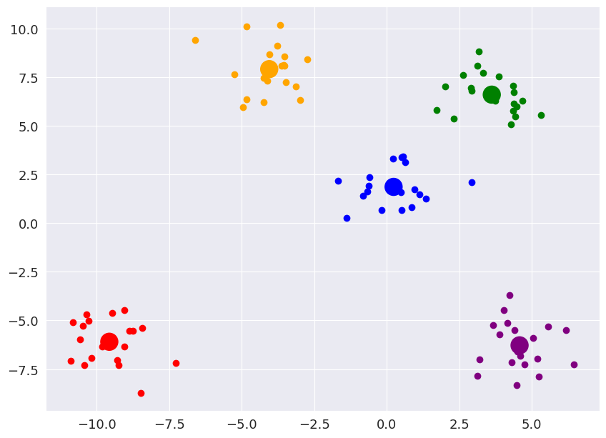
Example Data (for visualization): .png)
This was made using make_blobs of sklearn for ease of recreation and visualization.
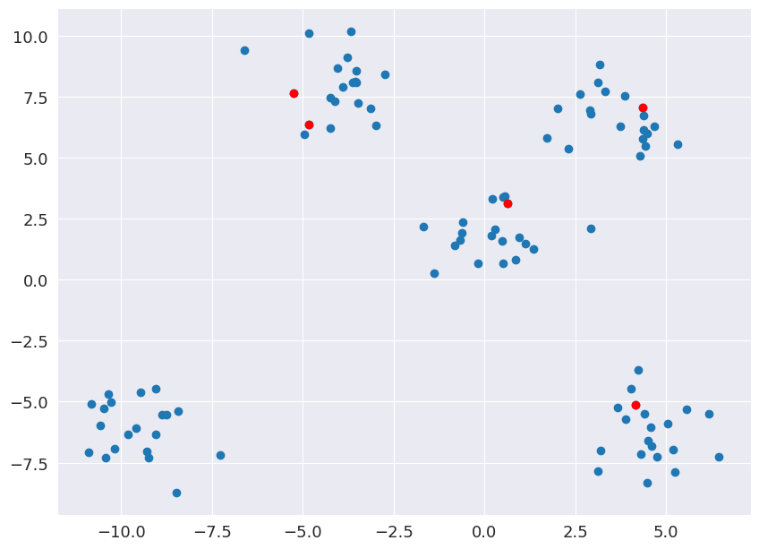
Step 1: Initialize ‘K’ random centroids
Not a great initialization as the upper left centroids are too close to each other. This can be fixed by using K-mean+ initialization that places centroids with the aim of maximizing the distance between them.
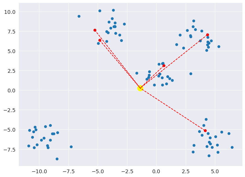 Step 2: Get the distance from each point to the centroids
This is repeated for each data point. In this example, yellow point is the closest to the centroid near the middle of the graph.
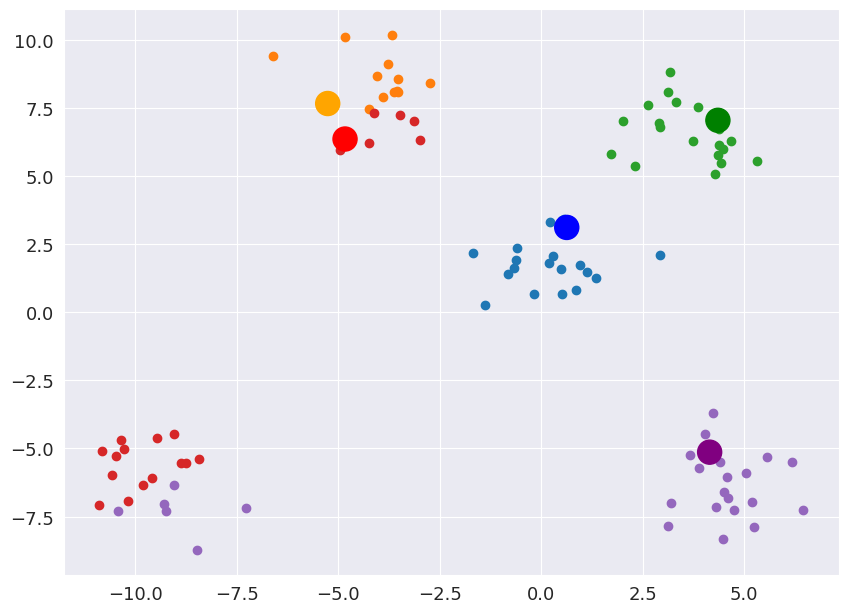 Step 3: Assign each point to a centroid based on minimum distance
The big points are the centroids and all data points are assigned and colored accordingly.
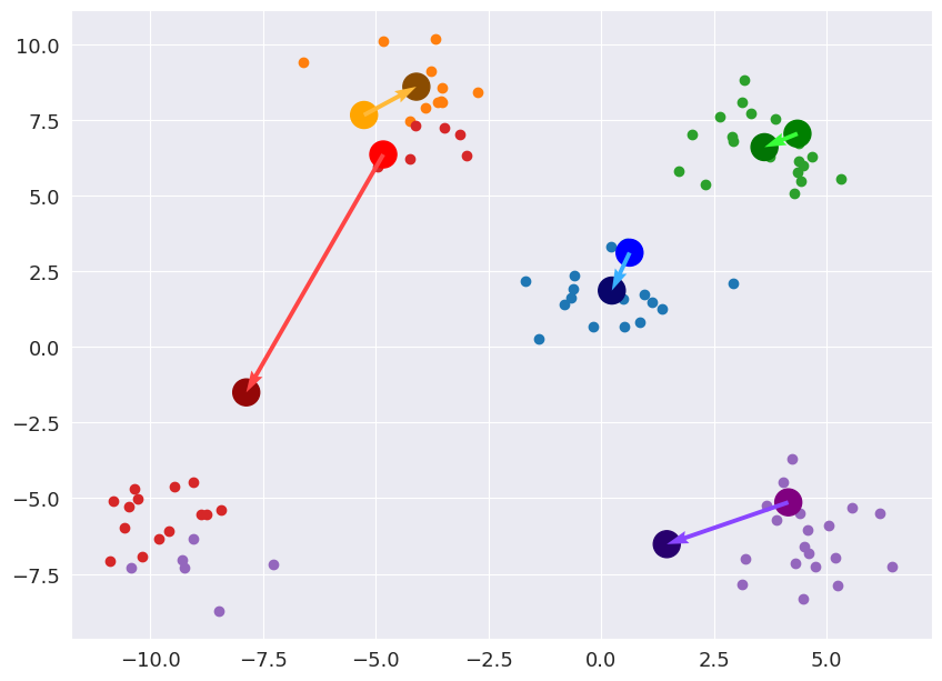 Step 4: Update the Centroids to the average of the cluster Now, we shift the centroid to the average of the current cluster.
 Step 5: Repeat steps 2–4 until the centroid keeps changing or till ‘n_iter’ Iterations
After the iterations, final resulting centroids and their respective clusters are shown below.
How to Evaluate?
Now that we understand the steps of K-means and how the clusters are formed, we can jump into the main topic of this blog! That is, evaluating the results of our algorithm.
Method 1: WCSS and elbow method
As we don’t have ground truths of the input data, we need another way to determine if the formed clusters are good enough.
Let’s take a step back, and analyze data in 1-D to get the picture.
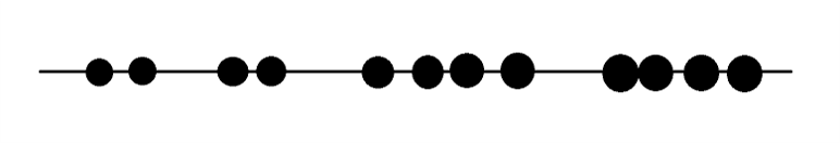
Here we have a few data points aligned in a straight line, and our aim is the same. Form the most optimal clusters.
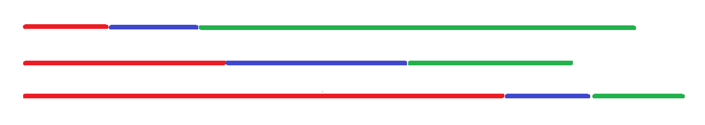
Here’s a few options for you. Which option do you think forms the best clusters.
Now, obviously it’s B. But why?
If we take the drawn lines and put them together as shown in the below figure, we can see that the line of option B take the smallest length.
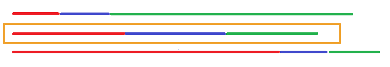
Now ask yourself, just what do these lines represent?
These lines are measuring the spread of the cluster. How the data point varies among the same cluster. As we know, as variance goes down, the similarity goes up. And the aim of our algorithm is to group similar data points together.
This will be the first way to evaluate cluster: Within Cluster Sum of Squares (WCSS).
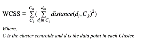
Formula might look daunting, but we are just iterating through each data point calculating the distance between it and it’s assigned centroid. Squaring and summing of distance is a very common way to understand the variance.
Let’s use this method on the clusters we formed using K-means. Now, one of the most important parameters of K-means algorithm is, well, K i.e. the number of clusters to be formed. In 2-D it might be relatively easy to understand and select a value of K. But this is near impossible for bigger dimensions (datasets with more features).
So let’s use this WCSS to determine the optimal value of our parameter K.
What we’ll do is, for each value of K, we will create clusters using K-means algorithm and record the Within Cluster Sum of Squares for each K value. Our next step is to simply plot the WCSS against the number of clusters (K) and we’ll get a graph similar to the one below.
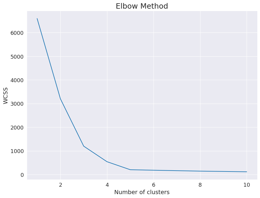
Here, we can see that there are a number of corners of the graph. The slope of the curve between K and K+1 values represents the impact that was made on the clusters by changing the K values from K to K+1. This kind of graph looks like an Elbow. Thus, this method of choosing K is also known as Elbow Method. And the most optimal value of K will be the corner of the elbow.
In our example, both K =3 and K=5 form decent corners for the visualized elbows. Most data scientists would infer here that K = 5 is more suitable as there is no significant decrease in WCSS after that.
Method 2: Silhouette Analysis
The next method to study is just as intuitive. Once we get the clusters from K-means, ideally we would want the average distance between the points of the same cluster to be minimum. This works well with our idea of grouping similar points together. Additionally, a point of cluster A should be as far as possible from the points in the next closest cluster. This last condition says that even the second closest cluster should be at a significant distance, thus, ensuring that other clusters are formed optimally.
A numeric variable that can predict how much of these two conditions is a cluster formation obeying, we have Silhouette Coefficient. It is the similarity of each data point to its own cluster (representing the cohesion) compared to its similarity with the next closest cluster (representing the separation).
The formula for this coefficient is given below.

Here, b(i) represents the average separation and a(i) represents the average cohesion.
If this coefficient comes out as +1, then b(i) must be far greater than a(i). This indicates that the sample is far from its neighboring clusters while being very close to its own cluster, thus satisfying both of our above defined conditions.
A coefficient value of 0, however, means that b(i) is very close to a(i), indicating that the sample is very close to the decision boundary between two clusters. Any value less than zero (<1) mean that samples have most probably been assigned to the wrong clusters, as the average distance to its neighboring cluster is less than the average distance to its assigned cluster. They can even be outliers.
Representation of cohesion — a(i)
.png) Representation for separation for the same sample — b(i)
Representation for separation for the same sample — b(i)
Understanding and comparing silhouettes:
As we did with the elbow method, we will use Silhouette Analysis to determine the optimal value of parameter K. Methodology remains the same, plot silhouette score for each value of K.
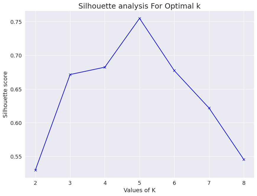
Silhouette analysis using the average of the score for the samples. A much better way to make a decision is to visualize the spread of the scores for each sample. In the following pictures, we have shown the distribution of silhouette scores for our dataset.
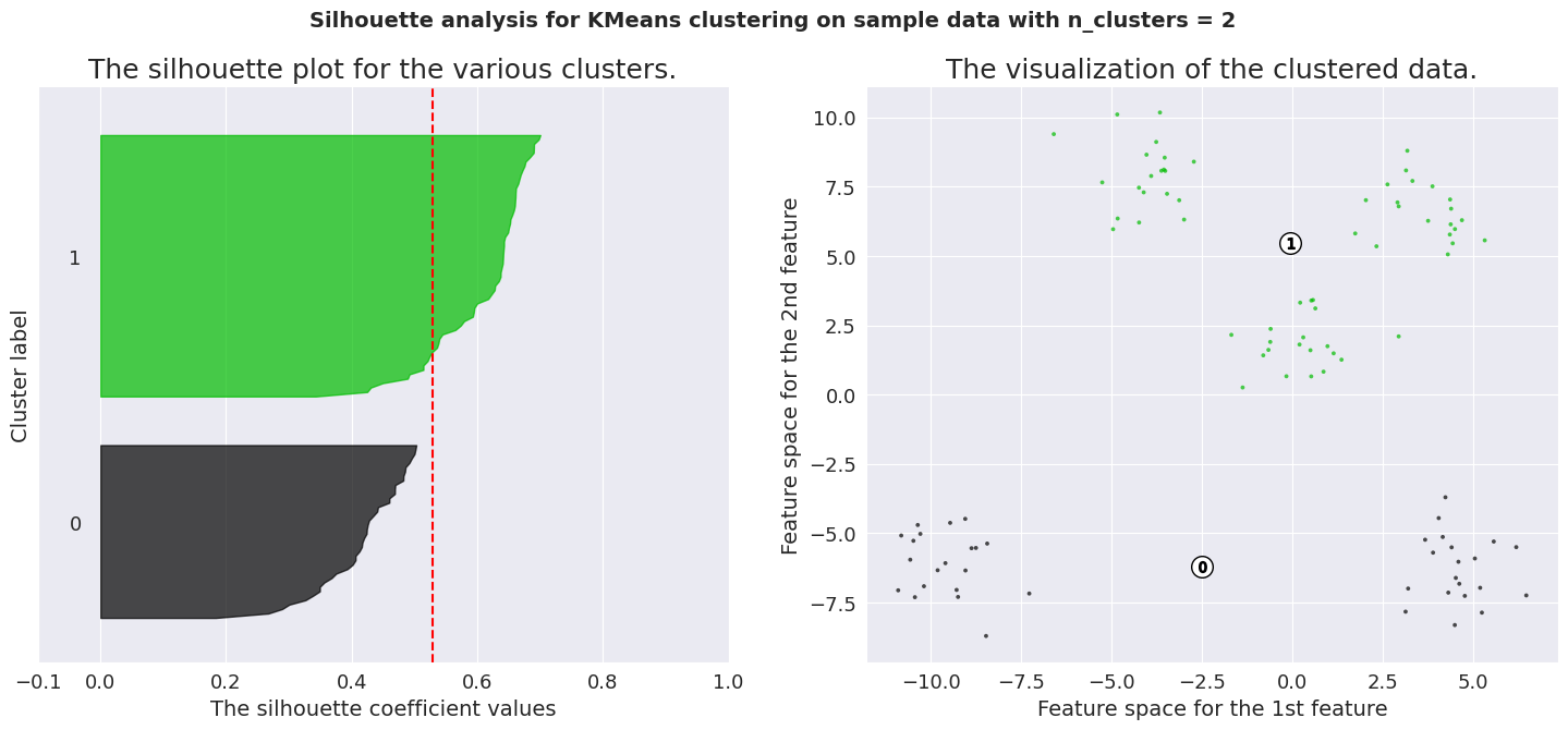
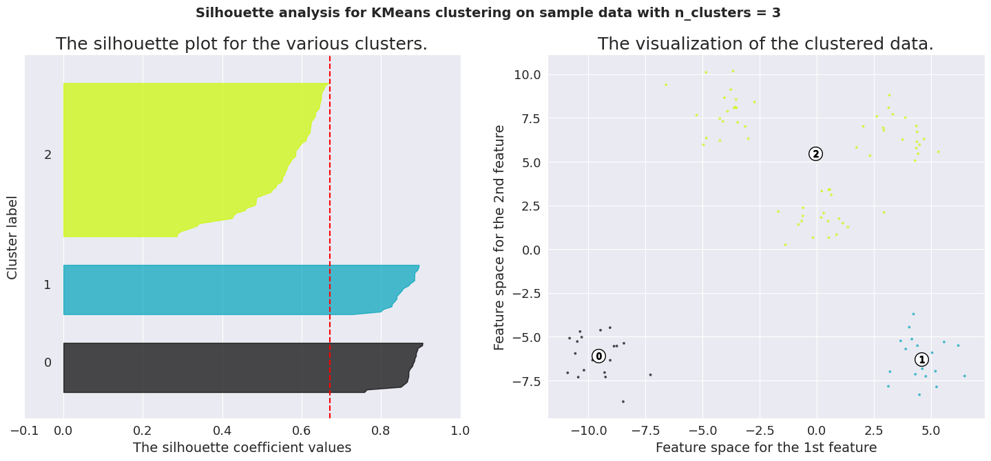
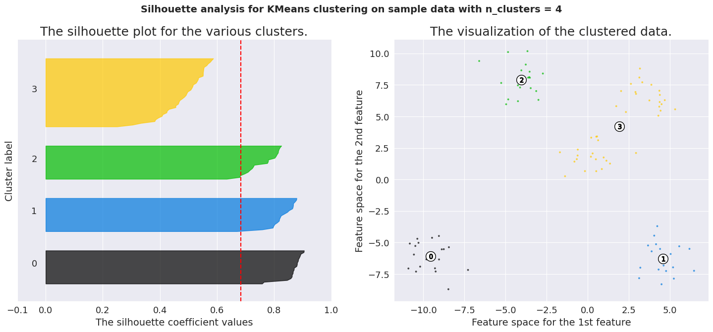
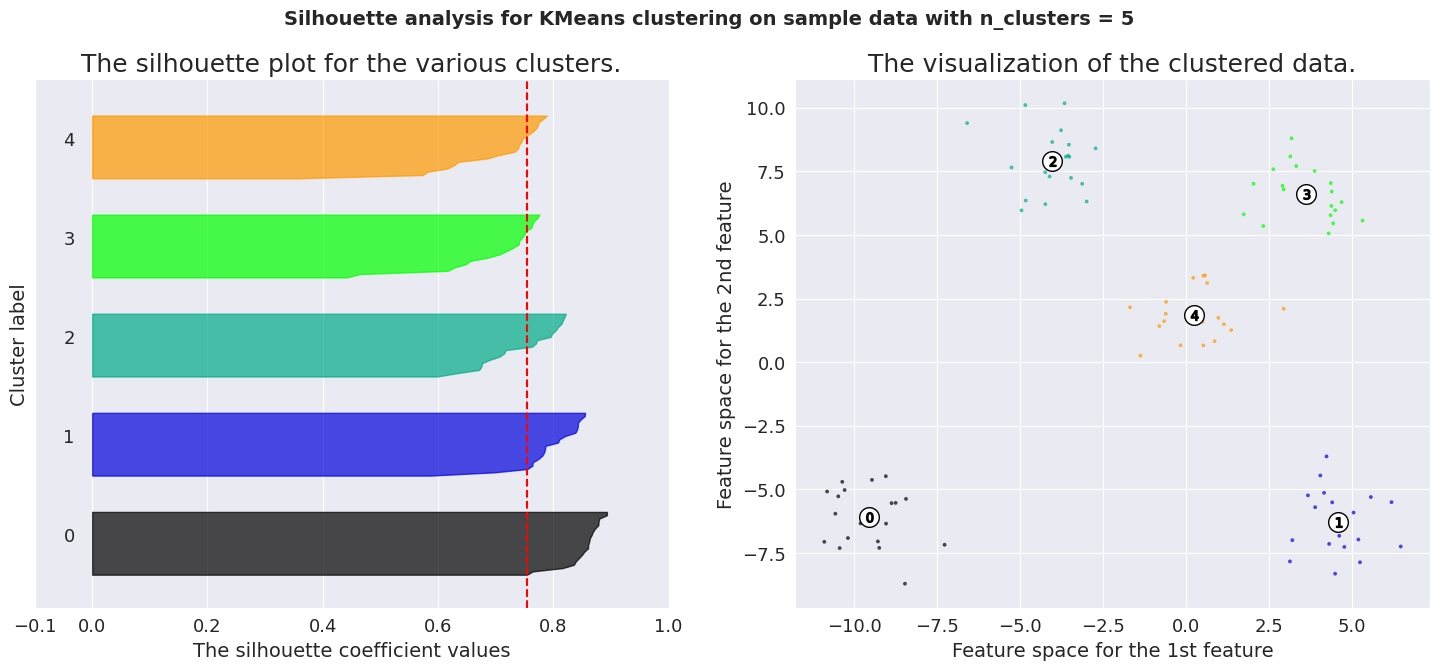
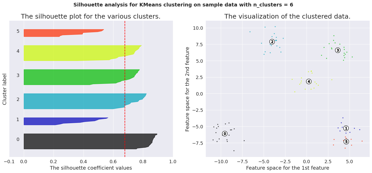
To analyze a silhouette plot like above, we need to observe 2 things.
Average silhouette score (represented by the red line) Similarity of the distribution for different labels The average silhouette score for K values 4, 5 and 6 are significant. But only the plots of K=5 are consistent across its clusters. This method is highly useful to detect any kind of outliers in the dataset.
Conclusion:
While there are many other methods to evaluate clustering algorithms, it is of utmost importance to understand the working and intuition behind these rather than just learning the commands. This is what will help you stand out from the crowd. With the intuition of these two popular methods, you can dive deep into the world of unsupervised learning explore even further beyond.
References:
Implement the above two methods: